Here is the midterm.
1. Hooke’s law says that the force required to stretch a spring a distance of  units from its natural length is given by
  where
where  is a constant that only depends on the spring.
We are told that for the spring of problem 1 we have  where units of distance are measured in meters, and forces in Newtons. This means that
  or
or  The work required to stretch the spring 10 m beyond its natural length is then
2. We are given a curve with equation  and asked to rotate about the
  -axis the segment where
  To find the area of the resulting surface, we can consider splitting the surface into little shells. A typical `thin’ shell, at height has surface area
  where
where  is the radius of the shell, in this case just the value of corresponding to
  i.e.,
i.e.,  Also,
Also,  is here the arc length element, given by
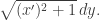
We have: 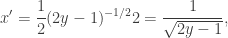 so
so 
Hence the requested area is given by 
This expression reduces to 
3. We are given the region bounded by the curve  and the lines
  and
and  We rotate it about the -axis, and are asked to find the volume of the resulting solid. A first attempt is to use the washer method. A typical thin washer consists of a slice of the solid for a fixed value of and with thickness
  Its volume is
  Here,
Here,  is the exterior radius, which in this case is always 2, and
  is the interior radius, given by
  This means the washer contributes
  of the full volume, and adding all of them together we obtain
  The upper limit of 4 comes from observing that the curves and cross precisely at the point
Unfortunately, this integral is not one of the given expressions.
So we attempt a different approach, using now the shell method. Now a typical thin shell is obtained by fixing a height and rotating about the -axis the slice of the figure of thickness  and height
  Its volume is
  where is the radius of the shell, in this case
  and
and  is the length of the shell, in this case
  We thus proceed to express in terms of
  Since
Since  then
then  Hence the thin shell contributes
  of the full volume, and the volume is obtained by adding all these contributions, obtaining
  This is expression (c).
4. The length of the curve  for
for  is given by the integral
  In this case,
  so
so 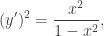 and
and 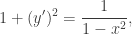 so the integral reduces to
  which is expression (b).
[There is a small problem with this integral, though, because the denominator vanishes at both endpoints. Later, in Chapter 7, we will learn how to handle integrals of this kind. Note that if the question had been to actually find the length, there is an easier method: The curve is half a circumference of radius 1, so the length is  ]
]
5. (a) The differential equation  can be rewritten as
  which is clearly separable. (T)
(b) The area swept by  for
for  is four times the area swept by
  Intuitively, we are making lengths twice as long, and areas carry two dimensions of length. Think of the area of a square of side 2, for example. Formally, we can check that this is the case: The area swept by the first curve is given by
 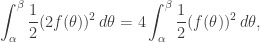 while the area swept by the second curve is given by
  (T)
(T)
(c) The half life of a given element is 3 days. This means that 50% of the given amount of the element has decayed after 3 days. After 3 more days, another 25% would have decayed. After 3 more days, another 12.5%. After 3 more days, another 6.25%. Since  the given statement is clearly true.
A longer way of checking the same is by recalling that the total amount of the element that remains after time  if originally the amount is
  is given by
  where is a given constant. Measure in days. We are told that
  so
so  Then
Then  and
and  (T)
(T)


 Posted by andrescaicedo
  is a formula, a generalization of
 are different or that they are present in
  )
) be a term, let
  be a variable, and let
  or
or  with
with  a variable occurring in
 whenever
  is a nonprincipal ultrafilter on the natural numbers, and
 for all
  or
or
 is a nonprincipal filter on a set
  then there is a nonprincipal ultrafilter on
  that extends
 Here, each
  is a constant symbol,
  is another constant symbol, and
  is a symbol for a binary relation (which we will interpret below as membership).
 A model
  of this theory
  would look a lot like
  except that the natural interpretation of
  namely,
  is no longer nonprincipal in
  is a common element of all these sets.
 thanks to the compactness theorem.
 let
let  and note that
 the thin slice of water in the tank at depth
  and weighs
  This is a constant force, so the work required to remove it to ground level is just
  where
where  is the depth at which the slice is located, i.e.,
  The total work is obtained by adding all these contributions, i.e.,
  ft-lb.
 Since
Since  the graph is symmetric about the
  is in the graph, then so is
  ).
). the graph is symmetric about the origin (because whenever
  ).
). Here
Here  so
so  which is impossible, so there is nothing to graph here. Consider now what happens when
  As
As  increases,
  increases, from
  to
to  So the same occurs with
  This means that
  , and
, and  decreases from
  The part with
  is undefined. This corresponds to the fact that at the origin the tangent to the curve is the
  Show:
Show:
 is definable (with parameters) and that
  Show that
  is finite.
 Show that there is some infinite
 Here,
Here,  is treated as a relation, and in
  we may have placed whatever functions and relations we may have need to reference in what follows; moreover, we assume that in our language we have a constant symbol for each real number. (Of course, this means that we are lifting the restriction that languages are countable.) To ease notation, let’s write
  for
for  The convention is that we identify actual reals in
  with their copies in
  so we write
  rather than
  etc.
etc.
 is a nonstandard model of the theory of problem 1. (In particular, check that the indicated restrictions of
  and
and  have range contained in
  )
) such that
  Otherwise, it is infinite. A (nonstandard) real
  but for all positive (finite) natural numbers
  We write
  to mean that either
  Show that infinite and infinitesimal numbers exist. The monad of a real
  such that
  which we may also write as
  and say that
  is an equivalence relation. Show that if a monad contains an actual real number, then this number is unique. Show that this is the case precisely if it is the monad of a finite number. In this case, write
  to indicate that the (actual) real
  We also say that
  is continuous at a real
  iff
iff  for all infinitesimal numbers
![{}[0,1].](https://s0.wp.com/latex.php?latex=%7B%7D%5B0%2C1%5D.&bg=ffffff&fg=333333&s=0&c=20201002) Argue as follows to show that
Argue as follows to show that  with
with  such that
  Conclude that the same holds if
  Let
Let  and argue that the maximum of
  then also
  Combined with the soundness Theorem
  and any formula
  if
if 