580- Topics in Set Theory. REMINDER

November 19, 2008

It is time to register, so please do not forget:

This Spring I will be teaching Topics in set theory. The unofficial name of the course is Combinatorial Set Theory. 

We will cover diverse topics in combinatorial set theory, depending on time and the interests of the audience, including partition calculus (a generalization of Ramsey theory), cardinal arithmetic, and infinite trees. Time permitting, we can also cover large cardinals, determinacy and infinite games, or cardinal invariants (the study of sizes of sets of reals), among others. I’m open to suggestions for topics, so feel free to email me or to post in the comments. 

Prerequisites: Permission by instructor (that is, me).

Recommended background: Knowledge of cardinals and ordinals. A basic course on set theory (like 502: Logic and Set Theory) would be ideal but is not required.

The course may be cancelled if not enough students enroll, which would make us all rather unhappy, so don’t let this happen.


175- Partial fractions decomposition

November 18, 2008

[This post replaces the previous version from October 12, 2008. The new argument is significantly simpler than the one originally posted.]

I want to present here a Calculus II-level proof that the method of partial fractions decomposition works. I will actually show a more general result, which will greatly simplify the presentation and get rid of most problems of the somewhat awkward formulation below. 

We need some notation:

  • \prod_{i=1}^n a_i means a_1\times a_2\times\dots\times a_n.
  • p(x), q(x), etc, denote polynomials with real coefficients.

The proof that I show below is algorithmic in nature, meaning that it provides us with a method to find the relevant constants for any given specific polynomials p and q. The constants we obtain are real numbers. 

That the method of partial fractions decomposition works means that we can always find the relevant constants the method requires.

Read the rest of this entry »


175 -A problem from Homework sets 9, 10

November 18, 2008

I want to show here how to solve the following problem from this week’s homework set: 

Starting with a given x_0, define the subsequent terms of a sequence by setting x_{n+1}=x_n+\sin(x_n). Determine whether the sequence \{x_n\} converges, and if it does, find its limit. 

This is a nice simple example of a (discrete) dynamical system in one variable. It turns out that the sequence always converges, but the limit depends on the value of x_0.

  • Case 1. x_0=n\pi for some n=0,\pm1,\pm2,\dots

In this case x_1=x_2=\dots=n\pi, so the sequence trivially converges.

  • Case 2. 2n\pi<x_0<(2n+1)\pi for some n=0,\pm1,\pm2,\dots

In this case I will show that x_0<x_1<\dots and that \lim_{i\to\infty}x_i=(2n+1)\pi.

First, notice that if 2n\pi<x_i<(2n+1)\pi, then we can write x_i=2n\pi+t for some t with 0<t<\pi and \sin(x_i)=\sin(t)>0, so x_{i+1}=x_i+\sin(x_i)>x_i.

Second, recall that \sin\theta<\theta for all \theta>0. You are probably familiar with this inequality from Calculus I; if not, one can prove it easily as follows: Let f(\theta)=\sin(\theta)-\theta, so f(0)=0. Also, f'(\theta)=\cos(\theta)-1\le0 for all \theta, so f is always decreasing, and the result follows.

Also, recall that \sin(t)=\sin(\pi-t), so

x_{i+1}=x_i+\sin(x_i)=2n\pi+t+\sin(t) =2n\pi+t+\sin(\pi-t)<2n\pi+t+(\pi-t)=(2n+1)\pi.

We have shown (by induction) that the sequence \{x_i\}_{i\ge0} is strictly increasing and bounded above (by (2n+1)\pi). Thus, it converges. If L is its limit, then

L=\lim_{i\to\infty}x_{i+1}=\lim_{i\to\infty}x_i+\sin(x_i)=L+\sin(L),

so \sin(L)=0 and since 2n\pi<L\le(2n+1)\pi, it follows that L=(2n+1)\pi. 

  • Case 3. (2n+1)\pi<x_0<(2n+2)\pi for some n=0,\pm1,\pm2,\dots

In this case, x_0>x_1>\dots and \lim_{i\to\infty}x_i=(2n+1)\pi.

The argument is very similar to the one for Case 2: If (2n+1)\pi<x_i<(2n+2)\pi, then \sin(x_i)<0 so x_{i+1}<x_i, and x_i=(2n+1)\pi+t for some t\in(0,\pi), so \sin(x_i)=-\sin(t)>-t and therefore x_{i+1}>(2n+1)\pi. It follows that the sequence \{x_i\}_{i\ge0} is decreasing and bounded below (by (2n+1)\pi), so it converges. As before, the limit must in fact be (2n+1)\pi, and we are done.


175, 275 -Homework 11 and suggestions for the week after Thanksgiving

November 18, 2008

Homework 11 is due Tuesday, December 2, at the beginning of lecture. The usual considerations apply.

In 175 we will try to cover this week until section 8.10, but probably won’t get that far. As mentioned last week,  we will also cover additional topics that the book doesn’t mention or doesn’t treat in sufficient detail, once we are done with 8.10. These topics are uniform vs. pointwise convergence (including Wierstrass test), the behavior of the p-series \displaystyle \sum_{n=1}^\infty\frac1{n^p} for p=2,3,\dots, and infinite products. I will distribute notes of the topics not covered in the book. If you want to read ahead, and would like some of the notes ahead of time, please let me know.

In 275 we will cover Chapter 14, probably this week we will cover until section 14.4. Particularly important are the notion of conservative field and Green’s theorem. Then we will continue with surface integrals and orientations, Stokes’s and the divergence theorems. This will probably take another week, maybe a bit more. If there is any time left afterwards, we will see Lagrange multipliers 

Homework 11:

175: Do not use the solutions manual for any of these problems.

  • Turn in the problems listed for Homework 10  that you still have pending.
  • Section 8.6. Exercises 8, 25, 28, 37, 60.
  • Section 8.7. Exercises 2, 4, 39-48. 

Besides the exercises you have pending from last week, there are 17 new problems. Turn in the exercises you have pending, and at least 10 of the new problems. The others (at most 7) will be due December 9, together with the additional exercises for that week. 

275:  

  • Turn in the problems listed for Homework 10  that you still have pending.
  • Section 14.1. Exercises 1-8, 12, 16, 29.
  • Section 14.2. Exercises 6, 8, 34, 41.
  • Section 14.3. Exercises 2, 6, 12, 17, 20, 34, 38.
  • Section 14.4. Exercises 2, 8, 18, 31-35.

Exercises 14.1.1-8 count as a single exercise. Besides the problems pending from last week, there are 23 exercises. Turn in at least 10 of these. The remaining problems (at most 13) will be due together with a few additional exercises on December 9.


A characterization of continuity

November 18, 2008

Yesterday, Randall Holmes mentioned to me the following nice characterization of continuity for functions between Euclidean spaces.

Theorem. A function f:{\mathbb R}^n\to{\mathbb R}^m is continuous iff it preserves path-connectedness and compactness.

This is an easy exercise, but I don’t remember having seen the characterization before, so I figured I could as well write down the argument I found. It is clear that the result holds for a much wider class of spaces than the {\mathbb R}^n, but to keep this post simple, I’ll just leave it this way.

Proof. For Euclidean spaces, continuity and sequential continuity coincide. Towards a contradiction, assume x_i converges to x but f(x_i) does not converge to f(x).

  • Case 1. The range of \{f(x_i): i\ge 0\} is infinite.

This quickly leads to a contradiction since \{f(x_i):i\ge 0\}\cup\{f(x)\} is a compact set: We may as well assume that the map i\mapsto f(x_i) is injective, and since f(x_i) does not converge to f(x) we may in fact assume that all the f(x_i) stay away from f(x). The set \{f(x_i):i\ge 0\} has an accumulation point, which cannot be f(x) so it must be f(x_m) for some m. But then the set \{f(x_i):i>m\}\cup\{f(x)\} is both compact and lacks one of its accumulation points, contradiction.

  • Case 2. The range is finite.

We may as well assume all x_i have the same image. Fix paths A_i=[x_i,x_{i+1}] in {\mathbb R}^n that we can combine to get a path \bigcup_i A_i\cup\{x\} (for example, A_i could simply be a segment). By preservation of path connectedness, any
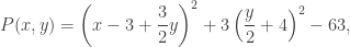
 A_i with range of size at least 2 in fact has range of size continuum. If infinitely many of the A_i have infinite range, one easily reduces to Case 1. So we may assume all the A_i have constant range, but then \bigcup_i A_i\cup\{x\} has a disconnected image. {\sf QED}


275 -Positive polynomials

November 11, 2008

When studying local extreme points of functions of several (real) variables, the textbook asks in one of the exercises to consider the polynomial

P(x,y)=x^2+3xy+3y^2-6x+3y-6.

Here we have P_x=2x+3y-6 and P_y=3x+6y+3, so the only critical point of P is (15,-8). Since P_{xx}=2 and the Hessian of P is 2\times 6-3^2=3>0, it follows that (15,-8) is a local minimum of P and, since it is the only critical point, it is in fact an absolute minimum with P(15,-8)=-63.

P being a polynomial, it is reasonable to expect that there is an algebraic explanation as for why -63 is its minimum, and why it lies at (15,-8). After all, this is what happens in one variable: If p(x)=ax^2+bx+c and a\ne0, then

\displaystyle p(x)=a\left(x+\frac b{2a}\right)^2+\frac{4ac-b^2}{4a},

and obviously p has a minimum at x=-b/2a, and this minimum is (4ac-b^2)/4a. 

The polynomial P of the example above can be analyzed this way as well. A bit of algebra shows that we can write

\displaystyle P(x,y)=\left(x-3+\frac32 y\right)^2+3\left(\frac y2+4\right)^2-63,

and it follows immediately that P(x,y) has a minimum value of -63, achieved precisely when both x-3+3y/2=0 and 4+y/2=0, i.e, at (15,-8).

(One can go further, and explain how to go in a systematic way about the `bit of algebra’ that led to the representation of P as above, but I will leave that for a future occasion.)

What we did with P is not a mere coincidence.  Hilbert’s 17th of the 23 problems of his famous address to the Second International Congress of Mathematicians in Paris, 1900, asks whether every polynomial P(x_1,\dots,x_n) with real coefficients which is non-negative for all  (real) choices of x_1,\dots,x_n is actually a sum of squares of rational functions. (A rational function is a quotient of polynomials.) A nonnegative polynomial is usually called positive definite, but I won’t use this notation here.

If Hilbert’s problem had an affirmative solution, this would provide a clear explanation as for why P is non-negative.

Read the rest of this entry »


175 -A curious series

November 10, 2008

I just learned from the textbook that apparently whether the series 

\displaystyle \sum_{n=1}^\infty\frac1{n^3\sin^2 n} 

converges is still open, which I find rather surprising. The reference the book lists is the book Mazes for the Mind by Clifford Pickover, St. Martin Press, NY, from 1992, but Dr. Pickover has informed me that he believes the problem is still unresolved; he also discusses it in his book The Mathematics of Oz, Cambridge University Press, 2002. I would be very curious to hear from updates or suggestions, if you have any.

Here is a slightly technical (and very quick, and not particularly deep) observation: The issue seems to be to quantify how small \sin^2 n is, when it is small, or more precisely, how sparse the set of values of n is for which the sine function is “significantly small.” One could start by looking at n so that |n-m\pi| is small for some m, so we are led to consider the standard convergent approximations to \pi, satisfying \displaystyle \left|\frac nm-\pi\right|<\frac1{m^2}. This means that 1/(n^3\sin^2 n) is close to, but slightly larger than, \displaystyle\frac{1/\pi^2}n, and so the question leads us to the problem of how sparse the sequence of numerators of the rational approximations to \pi actually is, something about which I don’t know of any results.

Below I display some graphs for the partial sums of the series. Let \displaystyle S(n)=\sum_{k=1}^n\frac1{k^3\sin^2 k}. The first graph shows n vs. S(n) for 1\le n\le 100. In the other graphs, n goes up to 300, 1000, and 100000. (Thanks to Richard Ketchersid for the code.) It is not clear to me that the last graph is accurate or that it allows us to draw any conclusions (it certainly seems to suggest that the series converges to a number slightly larger than 30); it may well be that further jumps are beyond the range I chose, or that the approximations Maple uses in its computations are not fine enough to examine very large values of the series.

Read the rest of this entry »


175, 275 -Homework 10 and suggestions for next week

November 10, 2008

Homework 10 is due Tuesday, November 18, at the beginning of lecture. The usual considerations apply.

In 175 we will try to cover this week until section 8.7 at least; it is possible this won’t happen until next week. Sections 8.3, 8.4, and 8.5 all introduce important tests for convergence of series; make sure you understand the arguments being presented (rather than just trying to memorize the tests). The material in section 8.6 is particularly important (conditional and absolute convergence). We will also cover some additional material on the p-series \displaystyle \sum_{n=1}^\infty\frac1{n^p}

Next week we will continue from section 8.7 (or at whatever point in the chapter we find ourselves at that point) on. We will also cover a few additional topics that the book doesn’t mention or doesn’t treat in sufficient detail, once we are done with 8.10. If you want to read ahead, the topics we will cover are uniform vs. pointwise convergence (including Wierstrass test) and infinite products. I will distribute notes of the topics not covered in the book.

In 275 we will cover from section 13.6 on, but the emphasis will be on section 13.8, and the notion of Jacobian. We will also present a few notions from linear algebra to make sense of the general version of the chain rule. Afterwards, we will continue with Chapter 14, which contains the main results from this course you are likely to use in the future. Chapter 14 will take some time to cover. 

Homework 10:

175: Do not use the solutions manual for any of these problems. 

  • Turn in the problems listed for Homework 9  that you still have pending.
  • Section 8.4. Exercises 3, 12, 23, 26, 35, 38, 40.
  • Section 8.5. Exercises 4, 8, 10, 25, 31, 34, 44, 47.

Besides the exercises you have pending from last week, there are 15 new problems. Turn in the exercises you have pending, and at least 7 of the new problems. The others (at most 8) will be due December 2, together with the additional exercises for that week. 
275:  

  • Section 13.5. Exercises 4, 8, 19, 22, 30, 45.
  • Section 13.6. Exercises 6, 11, 24, 30.
  • Section 13.7. Exercises 13, 21, 37, 60, 78, 79.
  • Section 13.8. Exercise 1, 6, 16, 21.

There are 20 exercises this week. Turn in at least 10. The remaining problems (at most 10) will be due together with a few additional exercises on December 2.


275 -Average values of harmonic functions

November 6, 2008

I want to mention here an important property of harmonic functions, the mean value property, and some of its consequences. I restrict myself to functions of two variables for clarity. 

Many important properties of harmonic functions (and, by extension, of analytic functions) can be established solely in the basis of the mean value property. I don’t know how to prove this property (or that it characterizes harmonicity) without appealing to Stokes’s theorem, or one of its immediate consequences (the topic of Chapter 14 of the book); in fact, I doubt such an approach is possible. It is a good exercise to see, at least formally, how this result gives the mean value property, but a rigorous treatment tends to be somewhat involved. Unfortunately, the arguments that show that the statements below hold tend to require techniques that are beyond the scope of Calculus III, so I will skip them.

Read the rest of this entry »


175 -The sine integral

November 5, 2008

The integral \displaystyle\int_0^\infty\frac{\sin x}x\,dx is an example of an improper integral: The integrand is not defined at 0, and the interval of integration is unbounded. The issue at 0 is not really serious, since

\lim_{x\to 0}\sin(x)/x=1.

Since the interval is unbounded, this integral is actually defined as a limit,

\displaystyle \int_0^\infty\frac{\sin x}x\,dx=\lim_{t\to\infty}\int_0^t\frac{\sin x}x\,dx.

In this post I want to show how to evaluate this limit. The problem is that the sine integral 

\displaystyle {\rm Si}(t)=\int_0^t \frac{\sin x}x\,dx

does not admit an elementary expression, i.e., it cannot be expressed in terms of t by composing exponentials, logarithms, trigonometric functions, their inverses, and polynomials.

(To get a sense of the difficulty in finding an expression for {\rm Si}(x), it may be useful to play a little trying integration by parts or similar tricks.)


Si(t)

This is a classical integral and appears in applications with some frequency, so there are several standard methods of computing its value. Usually, these methods involve techniques from complex analysis (either the Fourier transform or contour integrals), although there are some elementary approaches as well, such as the one I illustrate here. “Elementary” is to be taken with a grain of salt; although the argument below is easy to follow with some patience, it is difficult to come up with. There are good references where the integral is computed, but it usually takes me a while to remember where to look, so I decided to write this post and to provide a reference here as well.

An excellent book where the computation can be found more or less in complete detail (except for what I call Claims 1 and 2 below) is Introduction to Calculus and Analysis, vol. I, by Richard Courant and Fritz John, Interscience Publishers (1965), reprinted by  Springer (1989). The argument I present here is essentially the same they use, although I have arranged some of the details in a different way.

Read the rest of this entry »